


An Alternative Perspective for Framing the Gold Price Based on Fundamentals
This article was originally published in the ‘In Gold We Trust Report, The New Gold Playbook,’ in May 2024.
Get the fundamentals down and the level of everything you do will rise.
Michael Jordan
A fundamental based method for framing the gold price is presented along with a method for identifying its recurring support/resistance zones.
A simple tool for timing the gold price using the fed funds rate cycle.
The historical long-term cycle for gold suggests its ultimate peak is still 5 to 10 years out.
A case for a gold price target of USD 9,000 to USD 11,000 in the next 5 to 10 years.
The divergence between gold and TIPs based real yields can be interpreted as gold expressing a different opinion on inflation expectations.
Introduction
In the world of value investing, as the name suggests, understanding an asset’s valuation is fundamental to the approach. However, translating valuation to the gold market becomes tricky because the lack of cashflows precludes standard valuation methods. The question then becomes, what is the best way to understand gold’s value?[1] Many participants use technical analysis as their primary means through which to view it. However, what technical analysis lacks is an anchor that can fundamentally frame the value of gold throughout its cycles to something other than itself. Since gold has been a monetary asset for thousands of years, it is only natural to begin within that framework to best understand it. Starting from two simple assumptions, a richer and more fundamentals-based perspective on the gold price can be gained.
Assumption #1: Gold’s Relationship to Money Supply
Our first assumption is: The market value of the world’s investable gold supply (MVAu) is proportional to the market value of the USD money supply (MVM2).
From this simple assumption, a scaling relationship for the gold price can be derived that accurately tracks its long-term trend. Mathematically, this can be represented as,
which implies that gold’s scaled price into the future, G(t), can be expressed as,
By this method, a historical gold price, G(t0), can be projected through time using the growth in M2 money supply, gM2, and discounting by the growth in the world’s investable gold, gAu. Here we assume an gold supply growth rate, gAu, to be 1.5% per annum.

How does this help us to better understand gold’s value? It creates a convenient method to map out the various cycle levels for the gold price by projecting through time historical high-, mid-, and low-cycle levels for gold into the present by adjusting for embedded monetary inflation. For example, the post-revaluation gold price from 1934 of USD 35 per oz can be used as one such starting point. Here it is referred to as the cycle-high level since it only intersects the actual gold price near its long-term cycle highs, i.e. in 1934 and 1980. Other historical gold prices that represent mid-cycle and low-cycle levels can be similarly defined. Although this does not answer the question, “what’s the value of gold today?” it does provide a simple and fundamental-based method to frame where the gold price stands within its long-term cycle.

Recurring Support / Resistance Levels
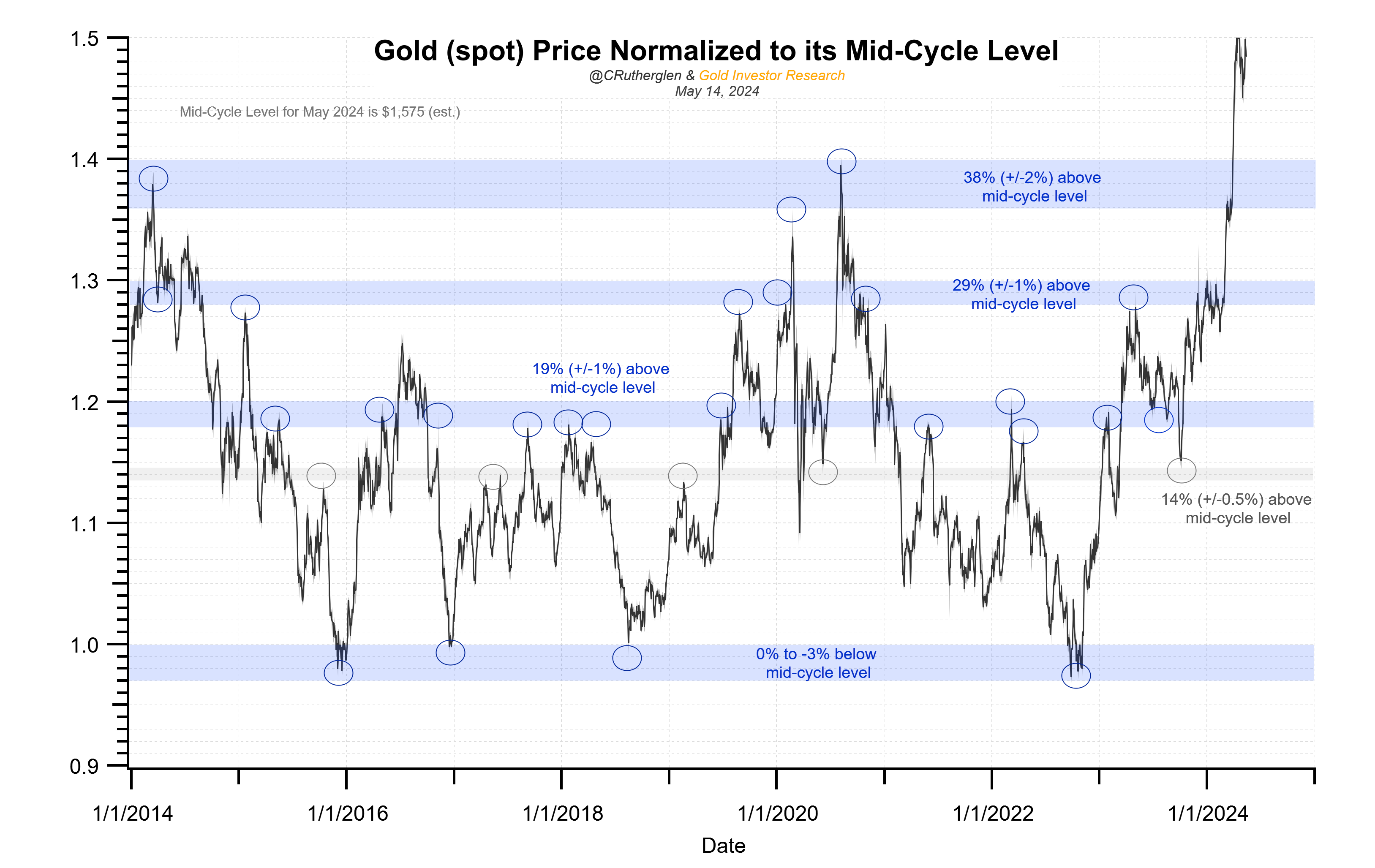
The utility of these long-term cycle levels does not end there. It turns out that some of them have had a tendency to reoccur as support/resistance zones going back nearly 50 years. This can be seen in the cycle chart above but even more clearly by normalizing, or taking the ratio of, the gold price to its mid-cycle level.
For example, the normalized gold price corresponding to 38% above the mid-cycle level has functioned as a major resistance level four times over the last 50 years: the December 1974 high, the November 1987 high, and most recently in the current bull market, the March 2008 and August 2020 highs. Then there is the mid-cycle level itself, which has functioned as long-term support. For example, in the past ten years, the gold price has rebound off of this level four times, including the important December 2015 and November 2022 lows.

In addition to half-century timescales, finer levels of recurring support/resistance can also be identified by zooming into the shorter periods. An example of this includes the level +19% above mid-cycle, which has experienced multiple tags as support/resistance over the past ten years. Mapping out and identifying these recurring support/resistance levels can be useful for gold investors to help target potential entry and exit points when the price gets near them. They can even be translated back into the gold price chart itself to complement more traditional technical analysis methods such as moving averages, etc. which we do at Gold Investor Research.
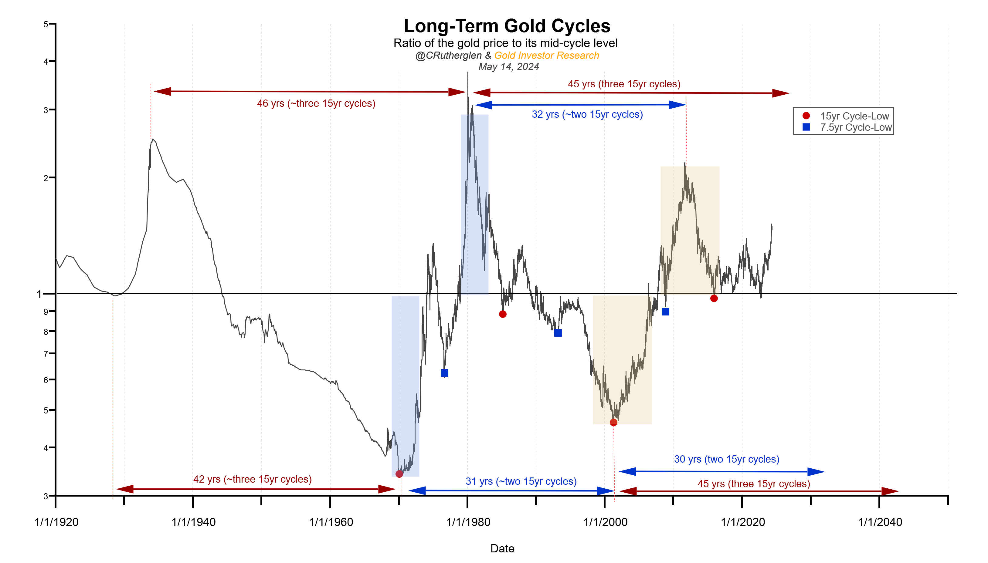
Zooming out to the very large 100-year timescale provides additional nuggets of information regarding gold’s long-term cycle. Since 1920, the gold price appears to have a long-term cyclical period of approximately 30 or 45 years. Interspersed within these are the more commonly known ~7.5- or 8-year cycles as well as the ~15-year cycles, which can be thought of as harmonics of the long-term cycle. Another important takeaway point is that, historically, the magnitude by which the gold price overshoots its mid-cycle level is about equal and opposite to the degree it undershoots it at the low. This was seen for the low-to-high period from 1970 to 1980 as well as in the period from 2001 to 2012.
Projections of Future Gold Prices
In addition to identifying potential near-term price targets, the framework can also be used to help explore where gold price cycle levels may be in the future. Leveraging gold’s relationship with the quantity of money, if an opinion can be expressed on where US money supply is likely to trend, then it is straightforward to project a cone of possibilities on where the gold price cycle levels may be at some future date.
One approach to help quantify this using first-order analysis is to observe that from 1915 to 1978, the ratio of United States all-sector debt securities and liabilities to M2 money supply was fairly stable around an equilibrium level of 2.5. In other words, during both the interwar and Breton Woods monetary periods, the US economy functioned well with one unit of money supply supporting ~2.5 units of debt. From the late 1970s to the GFC in 2007/2008, debt expanded much quicker than money supply, pushing the ratio up to a peak of 7 units of debt supported by one unit of money supply.
This high relative level of debt was presumably unsustainable, because immediately following the GFC, the Federal Reserve radically changed their monetary policy and began growing the money supply at over twice the rate of debt, primarily via their new quantitative easing (QE) programs. Since then, the debt-to-money supply ratio has been on a general downward trend with a small countercyclical upswing in the past year or so as the money supply has contracted. If it is assumed that the ratio will continue on its general path towards the ~2.5 level, then a corresponding range of expectations can be set on where the gold-cycle levels may be. For example, assuming all-sector debt securities & liabilities continue to grow at around 5% per year, then an M2 money supply of USD 50trn or USD 65trn would be needed for the ratio to regain the 2.5 level in the next 5-year and 10-year periods, respectively. This would translate into a gold price cycle-high level of approximately USD 9,000 and USD 11,000, respectively.

Assumption #2: Gold’s Relationship to Real Yields
Our second assumption is: The gold price is inversely proportional to real yields.
Although is well acknowledged that the gold price and the Treasury inflation-protected securities (TIPs) based 10yr real yield have had a fairly consistent inverse relationship, few take the analysis beyond that point to understand the relationship at a potentially more fundamental level. By digging deeper, an explanation can also be put forward as to why the broadly observed divergence developed between the two and what it may portend. To do so, it is useful to reframe the gold price from its dollar value into a real-yield equivalent, yreal,au, thereby putting gold on an equal footing with that of yields.

The inverse correlation between real yields and the gold price can be mathematically expressed in continuous compounding terms as:
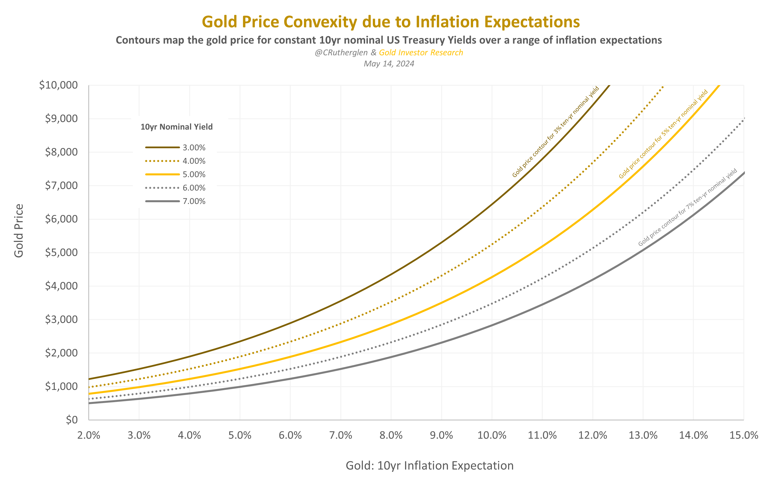
Within this framework, the gold price, G, takes the same form as a zero-coupon bond with a time to maturity, T, compounding based on a real yield, yreal,Au, and with a coefficient C that is similar to the principal for a bond. But unlike in the case of bonds, this coefficient C is not always constant but is subject to adjustments higher due to the cumulative effects of inflation. The other difference is, since gold obviously has no maturity date like a bond, it is more appropriate to refer to T as gold’s real duration, which based on the fitting is equal to approximately 22.4 years. In the case of a zero-coupon bond, its time to maturity and duration are the same since the only cash flow payment is at maturity. In practical terms, this means that the gold price has a lot of leverage – or convexity – to changes in real yields, similar to how long-maturity bonds also have a lot of price leverage to changes in nominal yields.
From 2008 to 2022, the gold-based real yield, yreal,au, was roughly equivalent to the TIPS-based 10yr real yield, yreal,TIPs, which is why the correlation was fairly strong. But starting in early 2022, the two began to diverge. Why?
There are likely two reasons. To address them, it is helpful to break out yreal,Au into its component form.
In lieu of a ~23 year zero-coupon bond yield as an input, the 10yr Treasury note yield, y10, is used due to its high liquidity, long time series, and the fact that we are comparing it to the 10yr TIPS. Since both the gold price and the 10yr yield are known, the only unknown is the derived gold-based inflation expectation, iAu. In other words, the entirety of changes in the dollar gold price that are not due to the 10yr yield can be captured in the term iAu. This shows that the divergence between the gold-based inflation expectation and TIPS 10yr breakevens began in March 2022 just as CPI inflation rate was nearing its peak. From then on, gold has been in a rising trend and clearly expressing a different opinion on inflation expectations than the TIPS 10yr breakevens do.

Large and increasing purchases of gold by central banks in the second half of 2022, as the divergence continued to widen, provide solid support that major market participants have been willing to pay this higher inflation expectation premium in order to gain exposure to gold. As of October 2023, the gold-based inflation expectation had continued trending higher and was implying a level just over 6%, even as the YoY CPI inflation rate had trended lower to just under 4%. Is this gold overshooting its inflation expectation, or is something else going on?
The possibility that something else is going on brings up the second potential contributing cause of the divergence, which is that the coefficient C may be in the process of resetting higher. Over the 2008 to 2022 period, when the correlation between TIPS- and gold-based real yields was strong, C was steady at approximately USD 1,525. Over the same period, gold’s fundamentals-based mid-cycle level, as discussed in the previous section, more than doubled from ~USD 750 to ~USD 1,600, meaning that the long-term cumulative effects of monetary inflation had embedded an approximate doubling in its price. As these cumulative effects continue to build, eventually they need to be reflected as a change in the coefficient.
During the first half of the 1970s, for example, C was much lower and likely closer to ~USD 80 in order to best fit the CPI inflation rate and the derived gold-based inflation expectation curves at the time. However, by the mid to late 1970s, the assumed correlation had increased to ~USD 200 or above. In the present inflationary environment, it may be that C is no longer constant and is going through one of its adjustments higher. If that is the case, there are two unknown variables, C and iAu, which makes disentangling their individual changes more difficult until a new steady state condition returns. A method does exist to overcome this limitation but is beyond the scope of this piece. For more on this, interested reads are referred to the article titled, “Towards a comprehensive framework for understanding the gold price: From 1971 to today.”
The Sweet Spot for Gold
Despite the shortcomings of using market-based real yields as a long-term valuation tool for gold, utility still exists in the gold real-yield-equivalent framework, since it identifies two primary drivers for the gold price, which are (i) falling yields and (ii) rising inflation expectations. This is not to say that every drop in the 10-yr Treasury note yield will produce positive returns for gold, since the two drivers can also work to offset each other. However, from 2000 to 2023, instances where the 10yr Treasury note yield declined by 15bp or more on the week produced a distribution of weekly returns for gold that is clearly positively biased, with a median value of +1.4%.

Not surprisingly, gold does its best during periods of persistently falling yields, which tend to occur late in the interest rate cycle, usually in anticipation of future rate cuts as the economy slows into a recession. For example, during advancing phases for gold, such as the current period from 2000 to present as well as in the 1970s, the gold price consistently reached an important local high midway through the Federal Reserve funds rate-cutting phase. This was seen at the gold price cycle highs in December 1974, March 2008, and March 2020 and is generally associated with the first half of a recession. Although the fed funds rate is not formally linked to the gold price through the gold real-yield-equivalent framework discussed above, in general, declining short-term rates are an anticipatory sign that the economy is slowing. Specifically, due to the time lag between the rate hikes and their actual effect on the economy, the inflation rate tends to remain elevated even as short-term rates are being cut.
This creates a sweet spot for the gold price because it provides the best of both worlds: that is, (i) elevated inflation expectations, and (ii) falling long-term yields as they price in lower future short-term rates. However, this sweet spot for gold that ultimately produces the cycle high is only temporary, because the time lags involved with the rate hikes ultimately do catch up with the economy. In the recession’s late stages, long-term yields begin to slow their rate of decline, thus removing a positive driver for the gold price, while inflation expectations themselves decline, which pushes the gold price down and ultimately to a cycle low. Examples of this include the October 2008 low during the GFC and the late-March 2020 low during the Covid shutdown.

Recent history has shown that in such an environment, the Federal Reserve and US Treasury typically step in with aggressive stimulus, which then sets the stage for an even higher gold price in the coming months and years. This secondary and more aggressive cycle high for gold has historically been driven by money supply expansion and rising inflation expectations, as seen in September 2011 and August 2020. Similarly in the late 1970s, when a second monetary impulse drove the gold price to ~USD 850 in January 1980. If the inflationary parallels between the current period and the 1970s were to play out and produce a second wave of inflation later in this decade, the trigger would likely be another money impulse near the end of the anticipated recession just ahead.

To summarize, if a similar dynamic were to roughly play out during the current interest rate cycle, the template could be:
First, the gold price breaks out of its 3.5 year consolidation pattern above USD 2,100 which did occurred 0n March 1, 2024.
Second, the gold price reaches a local-high (potentially up to USD 3,000) midway through the rate cutting phase driven by the ‘sweet spot’ of elevated inflation expectations and/or a declining 10yr Treasury Note yield. If the timing between the gold price breakout and its local-high were to follow the prior two interest rate cycles, it would suggest a high roughly between late-Q3 to Q4/2024.
Third, gold falls to a cycle-low and retraces much of the advance above the consolidation breakout level sometime in the late-stage of the recession, and
Forth, an aggressive move to an even higher cycle-high months to years later is driven by a presumed Federal Reserve and US Treasury stimulus action that is ostensibly meant to recover from the recession.
Conclusion
We have presented a framework for valuation/price analysis of gold that leans primarily on its fundamental drivers, which are (i) money-supply, (ii) inflation expectations, and (iii) long-term yields. It shows that a simple method exists to frame the gold price and identify its relative positioning within the long-term cycle.
Furthermore, viewing the gold price in a real-yield equivalent framework remains instructive for highlighting it primary drivers. Looking forward as the current interest rate cycle nears its end, history suggests the sweet spot for gold should emerge and take the gold price to a new local-high in 2024 roughly midway through the rate cutting phase. So far gold has indeed broken out of its 3.5yr consolidation pattern above USD 2,100 and is well on its way to the potential USD 3,000 target. Here we have shown that incorporating this alternative framework into an investor‘s tool-kit, it can provide a broader perspective and a more refined appreciation of how and when to best participate in this notoriously cyclical market and do so without solely relying on technical analysis.
[1] See also “The Synchronous Equity and Gold Price Model,” In Gold We Trust report 2022
Part II of this article is can be found at…
Towards a comprehensive framework for understanding the gold price

Previously we have shown that starting from two simple assumptions, a richer understanding of the long- and short-term trends in the gold price can be gained. To review, those assumptions were, ASSUMPTION #1: The market value of the world’s investable gold supply (MV